

Dynamic Mechanical Analysis Testing for Rubber and Elastomers:
- Home
- Dynamic Mechanical Analysis Testing for Rubber and Elastomers:
A Complete Guide for Process Engineers
How dynamic mechanical analysis (DMA) measures viscoelastic behavior across temperature, frequency, strain, and time, and how rubber labs use the data to qualify compounds, predict fatigue life, and feed simulation models.
SECTION 01
What Is Dynamic Mechanical Analysis for Rubber?
A compound passes every release test in the lab and fails in the field eighteen months later. An anti-vibration mount meets its stiffness specification on the bench and transmits noise at highway frequency. A seal qualified at room temperature goes stiff on the first chilly morning of the year. A tread compound ranks first in wet grip and last in rolling resistance, and nobody in the lab predicted the trade.
These failures share a cause. Rubber does not have one modulus. It has a modulus at a given temperature, at a given frequency, at a given strain amplitude, after a given loading history. Change any one of those four variables and the number changes with it, sometimes by orders of magnitude. Hardness, tensile strength, and compression set each report one value at one condition. None of them describes how the compound behaves at the conditions the finished part will see.
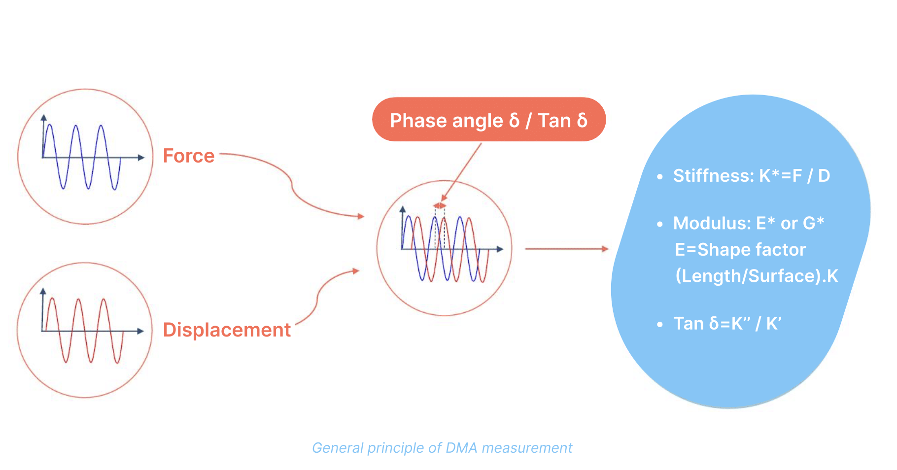
Dynamic mechanical analysis measures the full picture. A DMA test applies a sinusoidal excitation to a specimen at controlled amplitude and frequency, away from resonance, and records two signals: the applied force and the resulting displacement. From those two signals the instrument derives specimen stiffness, K* = F/D, and the phase angle ∂ between the force and displacement waveforms. Combine the stiffness with the specimen geometry and you get the complex modulus, E* in tension, compression, or bending, and G* in shear.
The complex modulus splits into two parts, and both matter for rubber.
Storage modulus (E’ or G’) is the elastic component, the energy stored during a cycle and returned when the load releases, and it governs dynamic stiffness.
Loss modulus (E” or G”) is the viscous component, the energy dissipated as heat, and it drives damping and heat build-up.
Tan ∂, the ratio of the two, is the damping factor. A purely elastic solid gives a phase angle of 0° and a purely viscous liquid gives 90°. Every rubber compound falls between the two, and where it falls depends on the test conditions. Unlike stiffness and modulus, tan ∂ does not depend on specimen shape, which makes it the most portable descriptor in the DMA data set.
DMA Guide Navigator
| If you need to... | Go to... | Key terms covered |
|---|---|---|
| Understand what DMA output means | Section 02 | E’, E”, tan δ |
| See where DMA fits alongside process rheology | Section 02 | RPA, ESR, complementary testing |
| Simulate real service vibration frequencies | Section 03 | Master curve, WLF |
| Test stiff, filled, or hard compounds reliably | Section 04 | Frame stiffness, force range, decades |
| Measure glass transition temperature | Section 05 | Tg, tan δ peak, DSC comparison |
| Predict fatigue life or crack growth | Section 06 | Tearing energy, crack growth rate, HBU |
| Qualify compounds across a temperature range | Section 07 | Temperature sweep, aging, cure state |
| Cut backlog or reduce operator dependency | Section 08 | Unattended testing, robotic handling |
| Feed FEA or digital twin models | Section 09 | Material model, linear domain, Prony |
| Meet a customer or regulatory specification | Section 10 | ISO, ASTM, reporting requirements |
| Compare or shop for an instrument | Section 11 | Buyer’s checklist, stiffness diagram |
Why rubber demands more from a DMA than rigid polymers do
Three properties of filled elastomers separate rubber testing from routine polymer thermal analysis.
- The modulus range is enormous. A compound in its glassy state below the glass transition sits three to four decades stiffer than the same compound on its rubbery plateau. Following the full variation inside a single temperature ramp needs a stiffness measurement domain of six to seven decades rather than the three to four and a half a conventional analyzer covers.
- The behavior is nonlinear. Because filled compounds exhibit both the Payne and Mullins effects, strain amplitude has to be controlled precisely and reported alongside every result.
- The service conditions are extreme. Rubber parts run from cryogenic sealing temperatures to under-hood heat, at frequencies from quasi-static creep to tire tread contact patch events well above 100 Hz, through millions of fatigue cycles.
Six Questions DMA Answers
Temperature sweeps map modulus and damping from cryogenic to high temperature and locate the glass transition and secondary relaxations.
Frequency sweeps and master curves extend characterization from quasi-static to 1000 Hz and beyond.
Controlled fatigue crack growth testing relates tearing energy G (strain energy release rate) to crack growth rate for lifetime prediction.
Aging studies, creep testing, and time-temperature superposition predict long-term behavior from short experiments.
Repeatable viscoelastic fingerprints detect formulation drift, incomplete cure, and supplier variation.
FREE DOWNLOAD
Introduction to Dynamic Mechanical Analysis
SECTION 02
Measuring Viscoelastic Properties of Rubber with DMA
Reading a DMA result starts with knowing which region of the viscoelastic spectrum you are looking at. Run a temperature sweep on any amorphous elastomer and storage modulus traces four regions: a glassy region where chain motion is frozen, a transition region where modulus falls two to three decades and tan ∂ peaks, a rubbery plateau where the crosslink network carries the load, and a thermal region where the network degrades. Most rubber parts operate on the plateau, which is exactly why the plateau alone tells you so little about failure. The interesting behavior sits at the edges.
Storage modulus at service temperature and service frequency sets dynamic stiffness. An engine mount specified on a static load-deflection curve behaves differently at 30 Hz, because rubber stiffens with frequency. Design a suspension component from static data alone and the vehicle rides harder than the model predicted.
Tan ∂ sets energy loss, and energy loss becomes heat. In a thick section under continuous cyclic loading, heat does not escape entirely; a part of it accumulates, raises core temperature, accelerates thermal degradation, and shortens fatigue life. A compound with attractive damping on paper turns into a heat build-up problem in a conveyor belt or a track pad.
The tire industry has built four decades of formulation practice on this relationship. Tan ∂ near 0°C correlates with wet grip, and tan ∂ near 60°C correlates with rolling resistance. A partial replacement of carbon black with silica raises the low-temperature peak, improving wet grip, while lowering tan ∂ at 60°C, improving rolling resistance. One temperature sweep shows both effects on the same curve.
Where DMA fits alongside process rheology
Rubber labs already run oscillatory shear rheology. A rubber process analyzer characterizes uncured compound: strain sweeps for filler dispersion through the Payne effect, frequency sweeps for the processability window, and cure curves for vulcanization kinetics. An encapsulated sample rheometer extends the same approach to polymers, prepregs, powders, pellets, and liquids at higher temperatures. Both answer the same category of question: how will this material process, and did it cure the way it was supposed to.
DMA answers the next question. It works on the cured part, in the deformation mode the part experiences, across the temperature and frequency range of service. It closes the loop between the formulation the compounder designed, the process the plant ran, and the performance the customer will experience.
Neither replaces the other. A lab running process rheology without DMA sends compounds out the door with no data on how they behave in use. A lab running DMA without process rheology diagnoses a performance problem with no visibility into where it originated.
| Rubber process analyzer (RPA) | Encapsulated sample rheometer (ESR) | Dynamic mechanical analyzer (DMA) | |
|---|---|---|---|
| Primary question | Processability and curing behavior | Melt behavior, Tg, viscosity, cure kinetics | Fundamental viscoelastic and mechanical properties |
| Material state | Uncured rubber compounds | Uncured polymer, prepregs, powders, pellets, liquids | Cured polymers, elastomers, plastics, composites |
| Deformation mode | Oscillatory shear | Oscillatory shear | Tension, compression, bending, planar shear |
| Temperature range | Roughly -60 to 230°C | Room temperature to 350°C | -150 to 500°C |
| Frequency range | 0.0016 to 50 Hz | 0.0016 to 50 Hz | 10-5 Hz up to 1000 Hz |
| Key outputs | Viscosity, G, S, tan δ, cure curve | Viscosity, G, S, Tg, tan δ | E*, G*, tan δ, Tg, aging, fatigue |
| Application focus | Mixing, processing, quality control | Mixing, processing, quality control | R&D, material selection, performance prediction |
SECTION 03
Frequency Sweep Testing and Master Curves
Almost every rubber specification in circulation reports properties at 1 Hz. Almost no rubber part operates at 1 Hz.
A running shoe sole sees 5 to 20 Hz. An anti-vibration mount works across 20 to 200 Hz. A tread element entering and leaving the contact patch experiences an event measured in hundreds of hertz. A conveyor belt over an idler, a rail pad under a passing axle, a seal in a reciprocating pump, all of them run somewhere other than 1 Hz. The gap matters because rubber properties shift with frequency the same way they shift with temperature.
The frequency effect, measured
An EPDM compound tested in compression on standard Goodrich cylindrical blocks, over a ramp from -60 to 100°C, gives different answers at different test frequencies. At 1 Hz the glass transition appears at -36°C. At 50 Hz the same specimen, in the same test, shows a glass transition at -27°C.
Nine degrees of Tg shift across one and a half decades of frequency. At low frequency the chains have time to relax and respond, producing more viscous behavior. At higher frequency they have less time, the response becomes more elastic, and the transition moves higher.
Now consider a cold-weather sealing specification qualified at 1 Hz on a part vibrating at 50 Hz in service. The qualification data says the compound is well clear of its transition. The part is not.
Frequency Effect on Glass Transition
What a 1 Hz qualification misses in an EPDM compound
The Problem
Qualifying vs Reality
The Solution
DMA Measurement
Why This Matters
Risk Reduction
The Result
Tested Compound
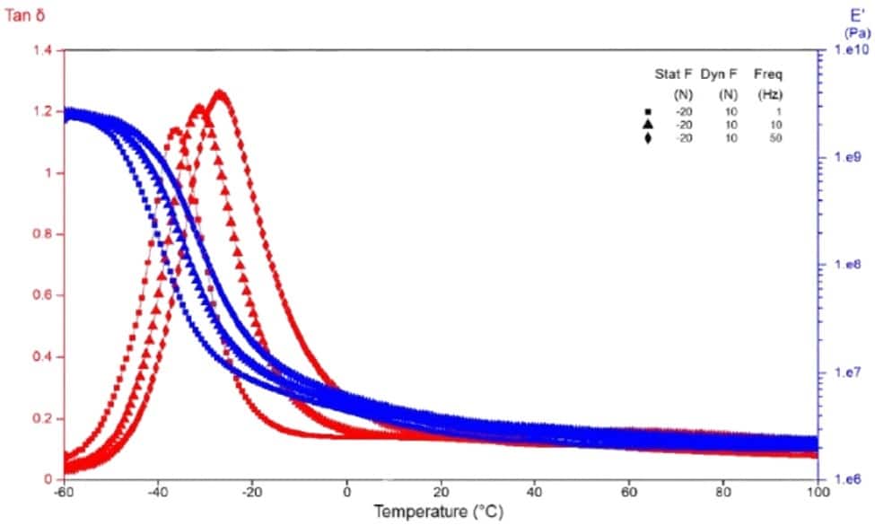
| Test frequency | Measured glass transition | What a 1 Hz qualification would have missed |
|---|---|---|
| 1 Hz | -36°C | Baseline |
| 10 Hz | -30°C | Transition moving toward service temperature |
| 50 Hz | -27°C | 9°C of margin |
Direct measurement versus extrapolation
Direct measurement runs frequency sweeps to 1000 Hz on a real specimen at a real temperature, given sufficient frame rigidity and appropriate shaker technology. No model, no curve fitting.
Time-temperature superposition runs sweeps at a series of stabilized temperatures, shifts each curve horizontally toward a reference temperature, and assembles a master curve covering a far wider range. Shift factors follow the Williams-Landel-Ferry relation near and above the glass transition, or an Arrhenius relation below it.
Master curves are useful and, for predictions above 1000 Hz, necessary. They also carry conditions, and rubber compounds break those conditions more often than rigid polymers do. Superposition assumes a homogeneous, isotropic, amorphous specimen with no structural change across the characterization range. It fails on block copolymers, on blends, on compounds crystallizing or partially melting in the test window, and on anything post-curing during the experiment. Build a master curve from a filled, blended compound without checking the assumptions and you get a smooth curve with no physical meaning.
Direct measurement over as much of the range as the instrument reaches shortens the extrapolation, and the shorter the extrapolation, the smaller the error it carries.
Four requirements govern a valid master curve. Run a strain sweep first, because superposition holds only inside the linear domain. Run a temperature sweep second, to locate the transition, since sweeps need close spacing through the region where E’, E”, and tan ∂ all vary steeply. Then run the sweeps themselves, typically 1 Hz to 100 Hz at fifteen or sixteen stabilized temperature steps. Finally, validate with a Cole-Cole plot, where loss modulus against storage modulus should trace a semicircle. Throughout, modulus should increase strictly with frequency and decrease strictly with temperature.
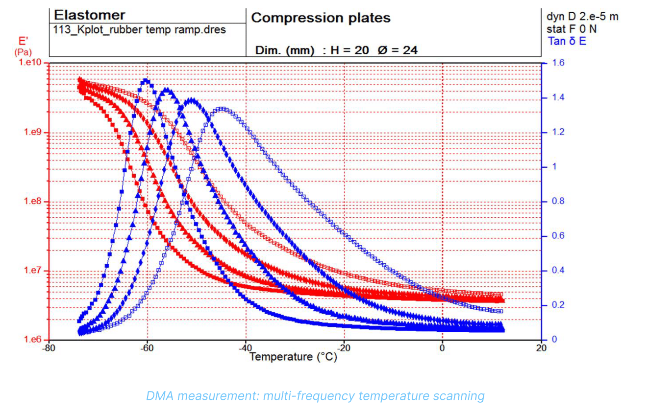
Multi-frequency temperature scanning
Running several frequencies simultaneously during one temperature ramp produces a family of curves without extending test duration. The technique earns its place for one reason. Primary relaxations shift with frequency. Secondary relaxations follow an Arrhenius law and do not shift the same way. Scanning multiple frequencies through one ramp separates the two on sight. A single-frequency ramp leaves you guessing.
RELATED CONTENT
CASE STUDY Building Frequency Temperature Superposition Master Curves
CASE STUDY Effect of Frequency on Viscoelastic Properties of Materials
SECTION 04
High-Force DMA and Testing Stiff or Filled Compounds
A DMA measures stiffness. Everything else – modulus, tan ∂, transition temperature – follows from a stiffness measurement and a specimen geometry. This single fact explains why some instruments produce clean data on a hard, filled compound at -60°C and others produce noise.
Frame rigidity sets the ceiling
The stiffness a DMA reports is not the stiffness of the specimen alone. It is the combined stiffness of specimen, holder, mechanical linkages, and instrument frame. When frame stiffness is much greater than specimen stiffness, the frame contribution disappears into the noise and the measurement reflects the material. When the specimen approaches the stiffness of the frame, you are measuring the machine.
Filled and hard compounds push against this ceiling constantly. Cool a carbon-black-filled or silica-filled compound through its glass transition into the glassy region and its stiffness rises three or four decades. Low-temperature qualification of rubber is the most demanding stiffness measurement a rubber lab runs, and it is where inadequate frame rigidity does the most damage, because the error grows exactly where the data matters most. A single-piece cast frame addresses this directly, removing the joints and interfaces where compliance accumulates in a fabricated frame.
Decades of measurement range, without a sensor change
The specification to look for is the stiffness measurement domain, expressed in decades. Conventional analyzers cover three to four and a half. Instruments built for rubber cover six to seven.
The difference shows up in workflow as much as in data quality. A narrow domain forces a transducer change partway through a campaign to stay in range, and every sensor change introduces a discontinuity where two halves of a data set stop being comparable. Holding one force-measurement chain across the entire range, with gains managed electronically, keeps a full temperature ramp on one metrological footing.
Every DMA has a measurable stiffness domain plotted against frequency, bounded above by frame rigidity and below by shaker technology. The specimen has to sit inside the envelope at every point in the test, which for a compound moving three decades during a ramp means at both ends. Ask any vendor for the stiffness-versus-frequency diagram before you buy. A vendor unwilling to supply one is telling you something.
Specimen size and measurement uncertainty
A 2% error in specimen dimensions produces a 10% uncertainty in the calculated modulus. Dimensional error is proportionally larger on small specimens, so specimen size is a direct lever on data quality. Tripling a specimen diameter cuts uncertainty on E’ by roughly a factor of 2.8.
Larger specimens are also more representative. A filled compound is heterogeneous at the scale of filler agglomerates and network structure. A specimen large enough to contain a representative volume describes the compound. A specimen small enough to sit inside one region describes one region.
Both arguments point the same direction, and both are limited by the force the instrument delivers and the space inside the thermal chamber. This is where force range stops being a data sheet number and becomes a constraint on what the lab is able to measure at all. It matters most for industrial vibration isolators, automotive bushings and mounts, aerospace elastomeric components, track pads, and any filled compound qualified for low-temperature service.
RELATED CONTENT
PRODUCT High force DMA+series
SECTION 05
Glass Transition Temperature Measurement in Rubber
Glass transition temperature is the most requested number in rubber DMA and the most frequently misreported. The difficulty is not measurement. It is Tg itself, which is not a single physical constant. It is a value derived from a curve by a chosen method at a chosen frequency, and two labs following different conventions will report different numbers for the same compound while both are correct.
Three definitions, one specimen
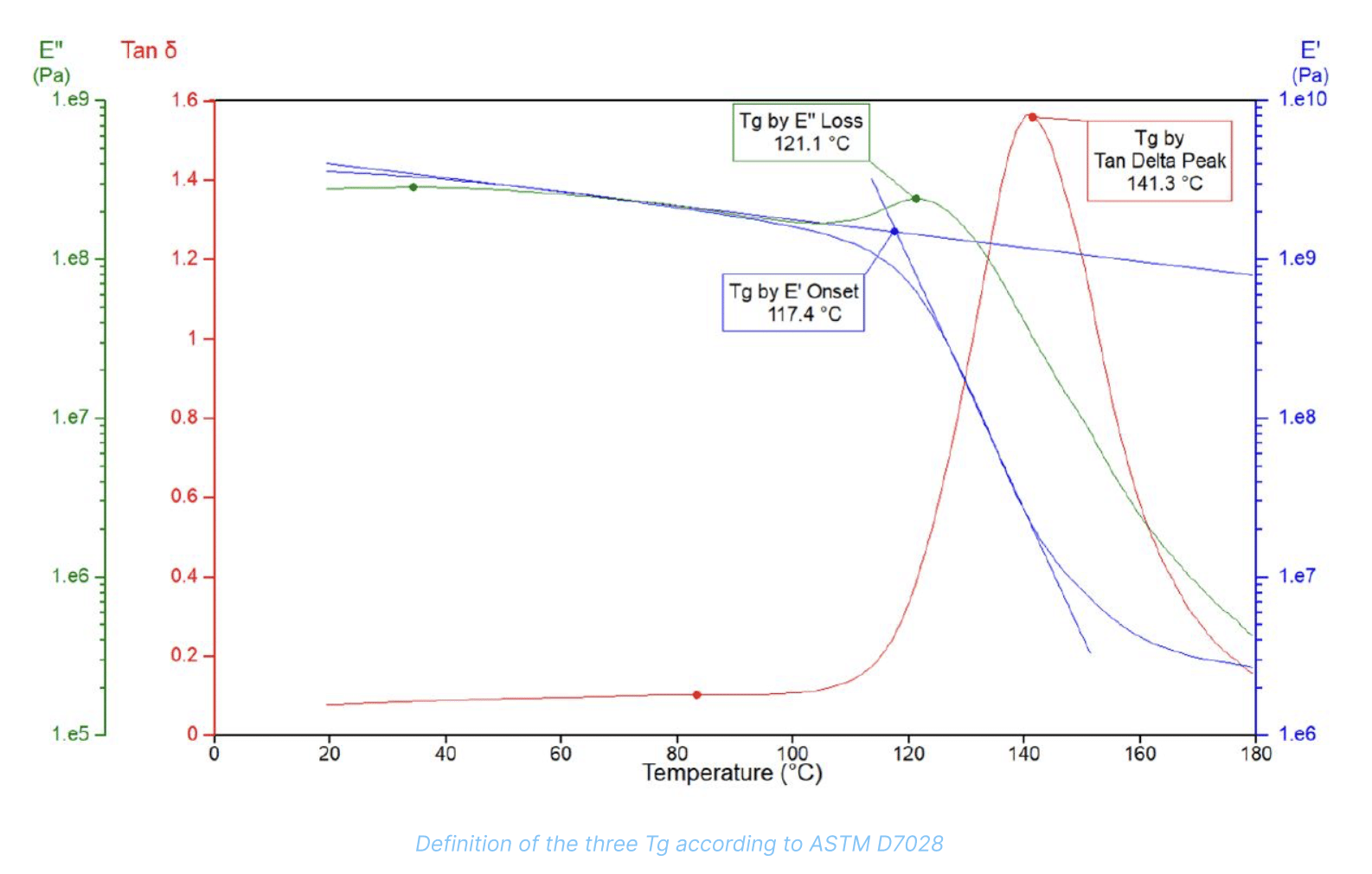
Onset Tg is the temperature where storage modulus begins its drop, the mechanical definition, and the one corresponding most closely to where a part starts losing the stiffness it was designed around. Tg by loss modulus is the E” peak, which at 1 Hz usually sits closest to a Tg from differential scanning calorimetry. Tg by tan ∂ is the tan ∂ peak, the chemistry definition, and the highest of the three.
On one epoxy example the three methods gave 117.4, 121.1, and 141.3°C. Twenty-four degrees separate lowest from highest, on one specimen, in one test.
The operational rule follows directly. Never report a DMA Tg without the method and the test frequency. A specification calling for a Tg is incomplete until it names both.
Tg depends on frequency, and DSC has no frequency
DSC measures a heat flow event. DMA measures mechanical relaxation, and mechanical relaxation depends on how fast you ask the question. The higher the excitation frequency, the higher the measured Tg. This explains most disagreements between a DMA result and a DSC result on the same compound. They are not measuring the same thing at the same rate, and neither is wrong.
Why DMA outperforms DSC on filled rubber
Sensitivity is the practical argument. DSC detects the transition as a step change in heat capacity, and in a heavily filled compound the polymer fraction generating the signal is a minority of the specimen mass, so the step is small, broad, and hard to locate reproducibly. DMA detects the same transition as a modulus drop of two to three decades and a clear tan ∂ peak.
DMA also resolves features DSC generally misses. Secondary relaxations below the glass transition appear as smaller tan ∂ features and govern low-temperature toughness. Multi-phase compounds resolve into separate transitions, one per phase, which is how a DMA trace detects a blend, contamination, or an incompletely reacted system a single-number test would pass.
Reach for DSC when the question is thermal: melting, crystallization, heat of reaction, residual cure exotherm. Reach for DMA when the question is mechanical: how stiff, how much damping, at what temperature, at what frequency. Most rubber labs need both.
Four practices separate a defensible Tg from a number nobody trusts. Hold the ramp at or below 2°C per minute, because faster ramps create a gradient between specimen surface and core. Verify the linear domain first with a strain sweep. Keep the thermal probe close to the specimen and in the same position every time, since probe position is one of the largest sources of lab-to-lab disagreement. Do not apply static displacement during a ramp, because thermal expansion turns a fixed displacement into an uncontrolled load.
RELATED CONTENT
APPLICATION NOTE Effect of Frequency on Viscoelastic Properties of Materials
SECTION 06
Fatigue Testing and Crack Growth Measurement in Elastomers
Most rubber parts do not fail because the compound was too soft or too stiff. They fail because a crack started somewhere and grew until the part came apart.
Conventional fatigue testing tells you when a specimen broke. Run enough specimens at enough load levels and you get a Wohler curve and a median life. What you do not get is the mechanism. You cannot tell whether compound A outlasted compound B because it resisted crack initiation or because it slowed propagation, and those two properties respond to entirely different formulation levers.
Servo-hydraulic testers and universal testing machines run into the same wall. They are built for component-level force, with load cells sized for kilonewtons, thermal enclosures large enough to hold a part, and frequency capability measured in tens of hertz. Precise control at low strain, accurate temperature regulation on a small specimen, and measurement of a crack tip position to micrometer resolution all sit outside their design envelope.
The controlled crack growth method
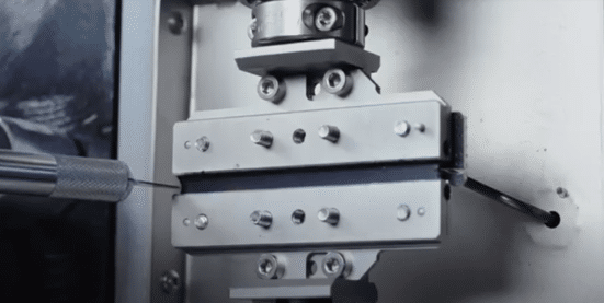 The approach in ISO 27727 measures fatigue crack growth rate of vulcanized rubber under repeated loading. A crack starts from a deliberate cut as shown here and grows progressively under cyclic load. The specimen geometry produces a pure tension conditions, and tests run at several tearing energies by varying strain amplitude. Specimens are molded strips, typically 40, 60, or 80 mm wide depending on how many cracks the lab follows at once, under 2 mm thick, with 6 mm between grips.
The test runs in three steps, and skipping any of them produces data nobody should trust.
-
1
Step one, stabilization. Applies a set number of cycles at the highest planned strain amplitude on an uncut specimen, removing the Mullins softening from the crack growth data.
-
2
Step two, characterization. Applies a strain sweep, still uncut, establishing the relationship between tearing energy G and strain amplitude.
-
3
Step three, crack growth. Follows a 5 to 10 mm razor cut, with crack tip position measured every 10,000 to 50,000 cycles at low tearing energy and every 2,000 to 5,000 at high.
The second step carries more weight than it appears to. Setting tests by tearing energy (strain energy release rate) rather than by strain is the step making results comparable between compounds of different stiffness. Two compounds tested at the same strain amplitude do not experience the same driving force at the crack tip. Two tested at the same tearing energy do.
Automated crack tip measurement
Excitation stops automatically after a programmed number of cycles. A static force opens the crack, a motorized camera targets each crack tip, real-time image processing returns the coordinates, every image is stored, and excitation restarts. The sequence takes about 15 seconds and requires no operator. Accuracy reaches 5 micrometers, matching an experienced operator with a microscope without tying anyone to the instrument for a multi-day test.
A cut at each end doubles the crack count, and adding a cut at the middle of a 60 or 80 mm specimen brings the total to four cracks in a single test, delivering reproducibility data in the same run rather than in three more of them. A reference point defined at the start gets checked before every measurement, so specimen slippage is detected rather than silently recorded as crack growth.
The primary output is crack growth rate, in nanometers per cycle, plotted against tearing energy, in joules per square meter. This relationship is the input to lifetime prediction, and it ranks compounds on the property driving field failure. It also captures effects a time-to-failure test would miss, since haversine and sine loading at the same frequency produce measurably different curves.
Heat build-up, the other fatigue mechanism
A heat build-up test applies static force to a cylindrical specimen and excites it continuously at fixed frequency and controlled strain, following the Goodrich flexometer approach. A thermocouple in an insulated plate tracks surface temperature throughout, and at the end a needle probe measures core temperature.
Both numbers are needed, and the gap between them is the finding. In one measurement the surface reached 66.57°C while the core reached 124.8°C. A surface measurement alone would have understated the thermal load by nearly 60 degrees. For a thick section under continuous cyclic loading, the core is where thermal degradation starts and where fatigue life is lost.
Testing Capability Table
| Test need | DMA capability | Output used for |
|---|---|---|
| Crack initiation resistance | Controlled cyclic loading from a defined cut, at set tearing energy | Compound screening, design qualification |
| Crack propagation rate | Automated crack tip imaging across cycles, up to four cracks per specimen | Fatigue life prediction, formulation ranking |
| Self-heating under load | Continuous surface temperature plus end-of-test core measurement | Thermal degradation risk, section thickness limits |
| Performance drift under load | Long-duration cyclic tracking of modulus and tan δ | Field failure investigation, aging correlation |
| Nonlinear response under cycling | Temporal signal capture and hysteresis loop analysis | Energy dissipation, Payne and Mullins characterization |
Fatigue crack growth and heat build-up arrive as modules on a DMA platform rather than as separate machines, and the crack growth optical stand retracts and pivots clear when the instrument returns to routine work. A crack growth capability specified at purchase and one added in year three deliver the same testing capability, and the second path lets the capital decision follow actual demand rather than a forecast.
RELATED CONTENT
SECTION 07
Temperature Sweep and Thermal Characterization of Rubber Compounds
A qualification built on room-temperature data describes one point in a service envelope spanning 150 degrees or more. Most qualification failures at temperature extremes trace back to a test program never run at the extremes.
The temperature sweep is the workhorse test in DMA and the first one to run on an unfamiliar material. A ramp at a controlled rate maps storage modulus and tan ∂ across the full service range and locates every thermal transition in it.
What a sweep reveals beyond Tg
Secondary relaxations. These appear as smaller tan ∂ features below the main transition and govern low-temperature impact resistance.
Blend structure. A two-phase system produces two transitions. A compound showing an unexpected second tan ∂ peak has a second polymer phase in it, by design, by contamination, or by incomplete mixing.
Cure state. This is the result most directly useful for quality control. Run a sweep on an under-cured specimen and it shows two tan ∂ peaks, one from the uncured fraction and one from the cured. The heat of the first ramp completes the cure. Run the identical test again on the same specimen and the lower-temperature peak has vanished, leaving a single sharper transition at higher temperature and higher amplitude. A third run superimposes on the second, confirming nominal properties. The diagnostic value is the comparison: two successive sweeps on one specimen tell you whether the part came out of the press fully cured, without a reference batch.
Aging, measured rather than assumed
A study on PVC specimens aged 12, 24, 50, 100, and 200 hours, tested in shear at 5 Hz from -50 to 150°C, produced a clear monotonic result. Shear storage modulus rose with aging time as the structure densified. Glass transition rose with it: roughly 65, 75, 82, 91, and 102°C.
Thirty-seven degrees of Tg shift from aging alone. Applied to a rubber part, this is the difference between a compound comfortably above its transition in cold service and a compound sitting on top of it. A hardness check on the same specimens would have reported the part got a little stiffer.
Creep and environmental conditions
A creep test applies static stress for a fixed time, measures the resulting strain, then releases and follows the recovery. Run at successive temperature stages within one test, creep data feeds the same time-temperature superposition machinery used for frequency master curves. One study on polypropylene ran 1800 second loading and recovery cycles from 15 to 95°C, and the resulting master curve predicts creep over several decades of time from an experiment run in a working day. For seals under bolt compression, mounts carrying static weight, or gaskets in a flange, ranking long-term dimensional stability from a short experiment is the difference between a design decision made on data and one made on a supplier’s assurance.
Rubber also rarely fails in dry air. A humidity module regulates relative humidity and temperature together, and on chitosan tested across 5 to 90 percent relative humidity, shear storage modulus fell by nearly two orders of magnitude. Liquid reservoirs allow testing while immersed in saline or oils at controlled temperature up to 80°C, and oxygen control from 10 ppm to 20 percent isolates oxidative aging from thermal aging.
Four practices govern a defensible sweep. Hold the ramp at 2°C per minute or slower. Match the temperature profile to the thermal mass of the system. Keep the thermal probe close to the specimen and in the same position across a campaign. Stay in the linear strain domain.
RELATED CONTENT
APPLICATION NOTE Effect of Aging on Mechanical Properties of Polymers
APPLICATION NOTE Curing Quality Control with DMA
APPLICATION NOTE Effect of Relative Humidity on Chitosan Polymer
SECTION 08
Solving Lab Throughput and Automation Challenges
Every lab manager reading this page has run the same arithmetic. A typical DMA test takes 30 minutes to 2 hours. An operator loads a specimen, launches the test, comes back when it finishes, unloads, and starts the next one. Nights and weekends contribute nothing. The constraint is not the instrument. It is the person standing next to it.
The productivity argument for automation is obvious enough to skip. The data quality argument gets less attention and is arguably the stronger one.
The operator effect is a measurement error, not an inconvenience
Consider one variable in specimen mounting: tightening torque. A single rubber compound, specimens of identical dimensions, one instrument, one test. The only change is the torque applied when clamping, at 0.5, 1.5, and 2.5 newton meters.
Storage modulus at 40 Hz came back at 1.54 x 10^7 Pa, 1.35 x 10^7 Pa, and 1.22 x 10^7 Pa. Higher torque, lower measured modulus. A 21 percent spread in the reported result, produced entirely by how tightly someone turned a screw. Tan ∂ was far less affected, which is one reason tan ∂ travels better between labs than modulus does, and cold comfort if the specification calls for modulus.
Now scale the problem. Two operators on two shifts. Three sites in a group comparing formulation data. A qualification campaign running six months with staff turnover in the middle. Every one of those transitions is a chance for a systematic offset to enter a data set and stay there, invisible, until someone tries to reconcile two labs’ results and cannot. Automated handling removes the variable. A robot applies the same gripping, loading, and clamping sequence to specimen 400 as to specimen 1.
What automated DMA looks like in practice
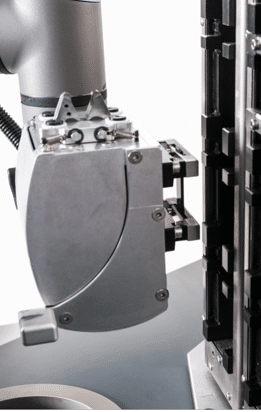
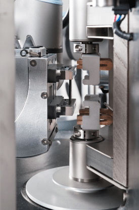
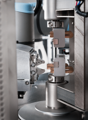
A six-axis collaborative robot arm removes a specimen from a carousel magazine, transfers it to the test station, loads it into the holders, closes the thermal chamber, and launches the test under the programmed conditions.
The carousel holds up to 12 removable racks, with capacity around 444 specimens in shear, 300 in compression, 120 in bending, and 108 in tension depending on specimen height. Racks load outside the system, so a running campaign never stops to be fed. Shear, compression, bending, and tension run on one machine and mix within one carousel, and reconfiguring between modes, or between automated and manual operation, takes under 15 minutes. The arm is collaborative, operating alongside personnel without a dedicated safety enclosure.
Two software behaviors do most of the practical work. Test chaining runs any sequence of DMA and fatigue tests automatically on a single specimen, a frequency sweep then a strain sweep then a temperature ramp, which also eliminates mounting variation between related tests. Operator alerts notify by text, email, or phone when a test finishes or stops unexpectedly, so the instrument does not sit idle overnight and a fault at hour six of a weekend campaign does not go undiscovered until Monday.
Continuous operation converts an eight-hour testing day into a twenty-four hour one on the same capital asset, and repeatability and inter-laboratory correlation both improve because operator-dependent variation is gone. The most valuable change is the least measurable: technicians stop loading and unloading and start interpreting results.
Capacity added to an installed instrument
Automation couples to an already-installed DMA in about two hours, without modification and without loss of original testing performance. The lab running a manual instrument bought three years ago and now facing a backlog is not looking at a replacement decision.
This is the practical shape of a scalable platform. Buy for the requirement in front of you. Add capability as the requirement grows. The instrument installed today keeps its full value when the lab’s needs change, which is a materially different proposition from a platform where the next capability means the next capital request.
RELATED CONTENT
PRODUCT Automated systems for DMA+ series
BLOG How to Conduct a Repeatability and Reproducibility (R&R) Test
FREE DOWNLOAD
Introduction to Dynamic Mechanical Analysis
SECTION 09
DMA Data for Simulation, FEA, and Digital Twins
Simulation groups working on rubber components need viscoelastic material models. Those models need data across the frequency, temperature, and strain range the component will see. When the data is thin, the model gets built anyway, on assumptions, and every prediction downstream inherits them.
The gap is rarely a modeling problem. It is a measurement problem, and it usually shows up as one of three things: data at one frequency when the model needs a spectrum, data in the linear domain when the component operates in the nonlinear one, or data with no traceable record of the conditions applied to the specimen.
What makes DMA data suitable for a material model
- Verified linear domain. A linear viscoelastic model is valid only where the material behaves linearly. Establishing the boundary takes a strain sweep before anything else. Data collected above it, fitted into a linear model, produces a model wrong in a way nothing downstream will flag.
- Wide, continuous frequency coverage. Prony series and other relaxation spectrum representations improve with the range and density of the data behind them. Direct measurement from quasi-static to 1000 Hz across a temperature range, assembled into a master curve, gives a fit anchored in measurement over most of its span rather than extrapolated across most of it.
- Correct shape factor and specimen sizing. Modulus is derived from stiffness through the specimen geometry. A 2 percent dimensional error becomes a 10 percent modulus error, and a 10 percent modulus error propagates through every stress and deflection the model predicts.
- Traceable excitation history. A single DMA data point is the end product of a sequence: a fade step to avoid overshoot, a stabilization step to accommodate the Mullins effect, a regulation step to reach the set point within tolerance, and an averaged measurement across a number of periods. Software storing the full history, including the regulation steps, lets a modeler verify the specimen experienced the nominal conditions. Software reporting only the final averaged value asks the modeler to take it on trust.
- Nonlinear characterization where the component demands it. Rubber components in service often work well outside the linear domain. Strain sweeps up and back capture Payne and Mullins effects. Stored temporal force and displacement signals produce hysteresis loops, which quantify energy dissipation per cycle and identify the transition between linear and nonlinear response. Hyperelastic and nonlinear viscoelastic models need this data, and it does not come out of a single-frequency temperature ramp.
Do not mix data from different instrument classes
Comparing data across instruments is one of the most common ways a good model gets built on a bad foundation. A DMA and a servo-hydraulic testing machine are not interchangeable sources, and combining their outputs into one data set produces a discontinuity in the middle of a material model.
The two are built for different jobs. A servo-hydraulic machine handles forces to roughly plus or -10 kN and is designed for components and industrial parts. Its temperature control is less precise, because the chamber is larger and the specimens are bigger. Low-strain testing is limited by the range of a large force sensor, and frequency capability stops at a few tens of hertz. What it does well is answer how a component performs.
A DMA handles specimens. It controls dynamic values precisely across the full strain range, regulates temperature closely on a small thermal mass, and reaches 1000 Hz. What it does well is answer how a material behaves and why, which is the input a material model needs.
Use each for what it was built for. If two dynamic data sets have to be reconciled, check the conditions applied to the specimen in each: the regulation history, the number of control loops, and whether any overshoot occurred large enough to have modified the material before the measurement was taken.
Getting the data into the workflow
Practical integration items worth checking during instrument selection: automatic determination of characteristic points such as Tg and tan ∂ peaks, customized and automated report generation, CSV export for spreadsheet and modeling workflows, and compatibility with the laboratory information management system the site already runs. A test result no one has to retype is a test result no one mistypes.
RELATED CONTENT
APPLICATION NOTE Building Frequency Temperature Superposition Master Curves
APPLICATION NOTE Creep and Time-Temperature Superposition (TTS)
SECTION 10
DMA Testing Standards and Compliance for Rubber
Published methods define specimen dimensioning rules, shape factors, excitation modes, and reporting requirements. They do not remove the operator’s freedom to choose geometry, frequency, ramp rate, and Tg convention, and the same compound tested under two defensible sets of choices returns two different numbers.
The implication for a lab manager: compliance with a standard is necessary yet not sufficient. A test program has to satisfy the standard and hold its own internal conventions constant, or year-over-year data stops being comparable to itself.
DMA Testing Standards
| Standard | What it covers | Why it matters |
|---|---|---|
| ISO 6721 (multi-part) |
Plastics: determination of dynamic mechanical properties. Part 1 general principles, with parts covering tensile, flexural, and shear vibration in non-resonance methods, and a part addressing glass transition | The reference method for specimen dimensioning rules and shape factors. Also the basis for the single-actuator requirement for applying static and dynamic excitation |
| ISO 4664-1 | Rubber, vulcanized or thermoplastic: determination of dynamic properties, general guidance | The rubber-specific counterpart to ISO 6721, written for elastomer test practice |
| ISO 27727 | Rubber, vulcanized: measurement of fatigue crack growth rate | The method behind controlled crack growth testing described in Section 06 |
| ISO 4666 (multi-part) |
Rubber, vulcanized: determination of temperature rise and resistance to fatigue in flexometer testing | Governs heat build-up test practice, including compression flexometer methods |
| ASTM D5992 | Standard guide for dynamic testing of vulcanized rubber and rubber-like materials using vibratory methods | The broad ASTM guide for dynamic rubber testing, covering method selection and reporting |
| ASTM D4065 | Plastics: determining and reporting dynamic mechanical properties | Defines reporting practice for DMA results, including the conditions to state with any value |
| ASTM E1640 | Assignment of the glass transition temperature by dynamic mechanical analysis | One of the two ASTM references defining how a DMA Tg is assigned |
| ASTM D7028 | Glass transition temperature of polymer matrix composites by DMA | Source of the three Tg definitions discussed in Section 05 |
| ASTM D623 | Rubber property: heat generation and flexing fatigue in compression | The Goodrich flexometer heritage behind heat build-up specimen geometry and practice |
Four common compliance gaps

Substituting shear rheology for a specification calling for DMA. A specification calling for tensile, compressive, or flexural dynamic properties on a cured part goes unsatisfied by a shear rheometer result, no matter how good the correlation looks internally.

Reporting Tg without the method and frequency. The single most frequent reporting failure.

Ignoring shape factor rules. Each excitation mode carries a recommended form factor. Tension needs height greater than twice the product of thickness and width divided by their sum. Planar shear for solids needs diameter greater than four times thickness. Three-point bending needs a span-to-thickness ratio above 8. Violating the rule produces a number the software will happily report and a modulus with no defensible relationship to the material.

Running an uncalibrated instrument. Drift of a few percent in either the force or the displacement channel produces an error of tens of percent in the reported modulus. Regular checks against a reference specimen of known stiffness, thermal checks against reference materials with known transitions, and annual calibration are the difference between traceable data and confident numbers.
FREE DOWNLOAD
Introduction to Dynamic Mechanical Analysis
SECTION 11
Choosing the Right DMA for Rubber Testing: A Buyer’s Guide
Instrument selection goes wrong in one of two directions. A lab buys for today’s requirement and discovers within two years the demanding samples, the ones driving the field failures, sit outside the instrument’s range. Or a lab specifies the largest configuration available to cover every scenario, pays for capability it will not use for five years, and defers the purchase for two budget cycles while it waits for the number to fit.
Both come from treating a DMA purchase as a single irreversible decision. It is more usefully treated as a platform decision followed by a series of capability decisions.
Specifications to evaluate
- Stiffness measurement domain, in decades. The most important specification and the least often quoted. A compound moving from rubbery plateau to glassy plateau spans three to four decades in a single ramp, so an instrument covering three to four and a half decades total has no headroom. Instruments built for rubber cover six to seven. Ask for the number and the stiffness-versus-frequency diagram behind it.
- Force range. Determines the largest specimen tested and the strain reached on stiff compounds. A constraint on data quality before it is a constraint on sample size.
- Frequency range. The floor matters as much as the ceiling. Quasi-static behavior supports creep and relaxation work, and the ceiling determines how much of the service range comes from direct measurement rather than extrapolation.
- Temperature range and cold source. A -150°C floor requires a cryogenic source, with liquid nitrogen carrying supply and safety overhead of roughly 5 litres per hour in continuous use. An air chiller reaching -70°C removes the supply chain entirely and covers the most frequently used range, which makes it the practical choice for continuous automated campaigns.
- Excitation modes and specimen holders. Elastomers test best in tension, compression, or shear. Bending suits high-modulus materials and produces noisy data on soft rubber. Confirm the holders exist for the geometries the lab receives in practice: cylinders, strips, films, cords, and specimens cut from finished parts.
- Environmental options, automation readiness, and upgrade path. Which capabilities are addable after installation and which are fixed at purchase. This determines whether the instrument bought today still fits the lab in year five.
- Software and data handling. Automatic characteristic point determination, full excitation history storage, automated reporting, CSV export, and LIMS compatibility.
Instrument category comparison
| Capability | Oscillatory shear rheometer | Servo-hydraulic tester | Dynamic mechanical analyzer |
|---|---|---|---|
| True viscoelastic data on cured parts | Limited | Limited | Yes |
| Tension, shear, compression, bending modes | No | Yes | Yes |
| Wide frequency range to 1000 Hz | No | No | Yes |
| Precise low-strain control | Yes | Limited | Yes |
| High-force testing of filled compounds | Limited | Yes | Yes, with adequate frame rigidity |
| Precise temperature control on a specimen | Yes | Limited | Yes |
| Glass transition determination | Limited | No | Yes |
| Fatigue crack growth measurement | No | Limited | Yes, with a crack growth module |
| Heat build-up measurement | No | Limited | Yes, with an HBU module |
| Unattended automated operation | Varies | Varies | Yes, with automated specimen handling |
When to consider an upgrade
Data becomes unreliable in the glassy region, or repeatability collapses at low temperature, meaning the instrument has run out of stiffness measurement range. The lab cannot reach the frequency the application needs, and every high-frequency answer arrives through an extrapolation nobody fully trusts. Backlog is chronic and a second shift is the only proposal on the table. A customer or a simulation group asks for data the instrument cannot produce. Support, calibration, or parts have become difficult to obtain.
Protecting the investment
Laboratory requirements move, and they rarely move in the direction the original justification anticipated. A lab buys a DMA to qualify compounds against a customer specification. Eighteen months later the simulation group needs master curve data. A year later a warranty investigation needs crack growth ranking. Another year on, volume has grown enough to make unattended operation the only way to hold the schedule.
On a fixed platform each of those becomes a capital request. On a scalable platform they are additions to an installed instrument. Automated specimen handling couples in about two hours without modification. Fatigue crack growth arrives as a module with a retractable optical stand pivoting clear for routine work. Heat build-up arrives as a dedicated holder with surface and core measurement. Cold sources, humidity control, immersion reservoirs, and controlled atmosphere are added when the application appears.
The purchasing consequence is worth stating plainly. Specify the platform against the most demanding sample the lab expects to see, because frame rigidity, stiffness measurement domain, and force range are fixed at purchase. Then add capability against actual demand rather than against a five-year forecast.
RELATED CONTENT
PRODUCT Desktop DMA series
PRODUCT High frequency DMA
SECTION 12
Key Terms
| Term | Definition |
|---|---|
|
Storage modulus (E’ or G’) |
The elastic component of viscoelastic response. The energy stored during a deformation cycle and returned when the load releases. Governs dynamic stiffness. |
|
Loss modulus (E” or G”) |
The viscous component. The energy dissipated as heat during each cycle. Drives damping and heat build-up. |
|
Tan ∂ |
The ratio of loss modulus to storage modulus, and the tangent of the phase angle between force and displacement. The damping factor, and independent of specimen shape. |
|
Specimen stiffness |
Applied force divided by resulting displacement. The quantity a DMA measures directly. Modulus is derived from it through the shape factor. |
|
Shape factor |
The geometric relationship converting measured stiffness into material modulus. Each excitation mode carries recommended rules in ISO and ASTM practice. |
|
Glass transition temperature (Tg) |
The temperature range where a polymer moves from a rigid glassy state to a softer rubbery state. Frequency dependent and reportable by three methods, so a value is incomplete without the method and frequency. |
|
Secondary relaxation |
A sub-glass transition linked to side-group and local chain motion. Follows an Arrhenius relationship and governs low-temperature toughness. |
|
Frequency sweep |
Measurement across a range of excitation frequencies at a stabilized temperature. Modulus increases with frequency. |
|
Temperature sweep |
Measurement across a temperature ramp at one or several frequencies. The primary tool for locating thermal transitions. |
|
Strain sweep |
Measurement across increasing strain amplitude. Establishes the linear domain boundary and characterizes the Payne and Mullins effects. |
|
Linear domain |
The strain range where modulus and tan ∂ stay constant with strain. Tg determination and master curve construction are valid only inside it. |
|
Payne effect |
The drop in storage modulus with increasing strain amplitude in a filled compound, caused by breakdown of the filler network. Relates to filler dispersion quality. |
|
Mullins effect |
The softening of an elastomer after the first deformation cycles, attributed to a reduction in effective elastic chains. |
|
Master curve |
A single curve covering a frequency range wider than direct measurement reaches, assembled by shifting sweeps run at different temperatures toward a reference temperature. |
|
Time-temperature superposition |
The principle behind master curve construction. Increasing frequency has the same effect on viscoelastic properties as decreasing temperature. |
|
Tearing energy (G) |
Also called the strain energy release rate, this is the energy driving a crack forward per unit area of new crack surface, expressed in joules per square meter. It is set by the strain energy density stored in the specimen, which the test controls through strain amplitude. Tear strength, the force to tear a piece apart, is a separate property under ASTM D624 measured in kilonewtons per meter. |
|
Crack growth rate |
The increase in crack length per loading cycle, in nanometers per cycle. Plotted against tearing energy for fatigue life prediction. |
|
Heat build-up (HBU) |
Temperature rise inside a rubber specimen under continuous high-strain cyclic loading. Measured at the surface throughout and at the core at the end. |
|
Frame rigidity |
The stiffness of the instrument’s test frame. It must greatly exceed specimen stiffness for the measured deformation to reflect the material rather than the machine. |
|
Stiffness measurement domain |
The range of specimen stiffness an instrument measures, in decades, plotted against frequency. |
SECTION 13
Frequently Asked Questions
Direct measurement versus extrapolation
What is DMA testing used for in rubber manufacturing?
Dynamic mechanical analysis measures how a cured rubber compound behaves across temperature, frequency, strain, and time. Rubber labs use it for compound qualification, glass transition measurement, damping and dynamic stiffness characterization, fatigue crack growth and heat build-up testing, aging and service life assessment, and generating the material data simulation teams need. The technique is non-destructive, so specimens remain available for further testing. See Section 01.
What is the difference between DMA and a rotational rheometer?
They test different material states. An oscillatory shear rheometer characterizes uncured compound in shear only: processability, filler dispersion through the Payne effect, and cure kinetics. A DMA characterizes cured material in tension, compression, bending, or shear, from -150°C to 500°C and up to 1000 Hz. Process rheology tells you how a compound will mix, flow, and cure. DMA tells you how the finished part will behave in service. Most rubber labs need both. See Section 02.
How does DMA measure glass transition temperature?
A temperature ramp produces three candidate values: the onset of the storage modulus drop, the loss modulus peak, and the tan ∂ peak. All three are recognized in standards practice, and they differ from each other, sometimes by more than 20 degrees on one specimen. Tg measured by DMA also depends on test frequency, rising as frequency increases. Always report the determination method and the frequency alongside the value. See Section 05.
Is DMA or DSC better for measuring Tg in rubber?
DMA is more sensitive on filled elastomers. DSC detects the transition as a step change in heat capacity, and in a heavily filled compound the polymer fraction generating the signal is small, producing a weak and broad step. DMA detects the same transition as a modulus drop of two to three decades and a clear tan ∂ peak, and also resolves secondary relaxations and the separate transitions of multi-phase compounds. DSC remains the better tool for melting, crystallization, and heat of reaction. See Section 05.
What is tearing energy in rubber fatigue testing?
Tearing energy, written G and expressed in joules per square metre, is the energy driving a crack forward per unit area of new crack surface. It is also called the strain energy release rate. It is not a force, and it is not the force needed to tear a specimen apart, which is tear strength under a separate method.
In a fatigue crack growth test, tearing energy is the controlled variable. The lab sets a level by choosing the strain amplitude, which fixes the strain energy density in the specimen, then measures how fast the crack advances at that level. Running several levels builds the relationship between applied tearing energy and crack growth rate, which is the input to lifetime prediction.
The pure shear geometry required by ISO 27727 holds tearing energy constant as the crack extends, so one test at one applied level yields one clean growth rate. Growth rate still differs from one applied level to the next, and mapping that dependency is the point of the method.
Matching applied tearing energy is also what makes compound comparisons fair. Two compounds of different stiffness tested at the same strain amplitude do not experience the same driving force at the crack tip. Two tested at the same tearing energy do. See Section 06.
Why do two labs get different DMA results on the same compound?
Several sources, in rough order of magnitude. Specimen mounting, where tightening torque alone produced a 21 percent spread in storage modulus in a controlled comparison. Test frequency, which shifts Tg. Excitation mode. Ramp rate and thermal probe position. Specimen dimensioning, where a 2 percent dimensional error becomes a 10 percent modulus error. Calibration drift, where a few percent in the force or displacement channel becomes tens of percent in the reported result. Automated handling, defined conventions, and regular calibration address most of it. See Section 08.
FREE TECHNICAL RESOURCE
Introduction to Dynamic Mechanical Analysis
A complete introduction covering measurement principles, instrument specifications, specimen sizing rules, and the main DMA test protocols.