

Introduction
High Frequency Needs
Nowadays, a lot of materials are submitted to repetitive mechanical force or solicitation. For example: some joint polymer part in a turbine system, or the surface of a tire repeatedly crossing the road. In order to characterize this kind of effect on the material, the DMA is one of the best tools.
Alpha Metravib DMA+ allows the study of specimens from high force range, high displacement and high frequency up to 1000 Hz. While the 1000 Hz range covers up the large majority of direct application from polymer material, studying the viscoelastic properties at higher frequency can bring specific information about the material behavior in certain circumstances.
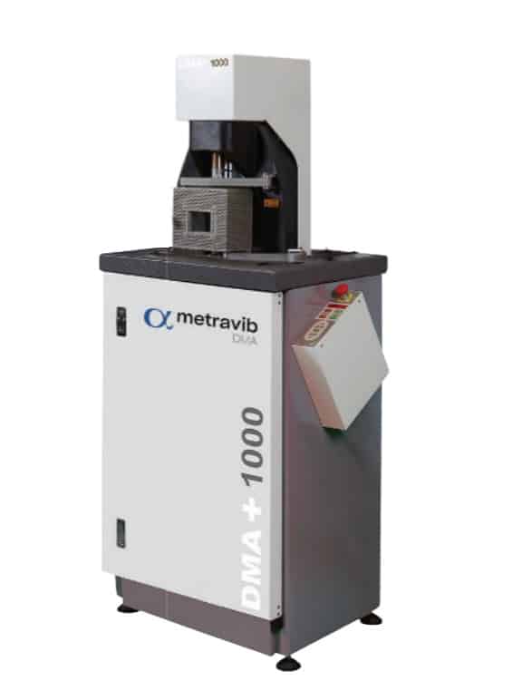
One of the best examples is to evaluate the grip of a tire or a shoe sole on some specific and flat surface. In those cases, the viscoelastic properties over 1000 Hz are of a key characteristic to predict how the car (or the runner in the case of a shoe) will perform on these surfaces.
Unfortunately, usual DMA cannot perform tests over 1000 Hz due to mechanical limitations.
FREE DOWNLOAD
Introduction to Dynamic Mechanical Analysis for Rubber Materials
Master Curve Principle
To overcome this limitation, the FTS (Frequency Time Superposition) is used to build Master Curves based on the WLF model (Williams–Landel–Ferry equation) or Arrhenius model.
The principle is quite simple. It is based on the fact that there is an equivalence between the frequency of the mechanical solicitation and the temperature in the viscoelastic properties of a material. This principle is illustrated in Figure 2 with a fictitious representation of two frequency sweep tests performed at 10°C and 30°C between 1 Hz and 100 Hz: the modulus of elasticity shows the same value at 10°C from 1 Hz to 10 Hz as at 30°C from 10 Hz to 100 Hz.
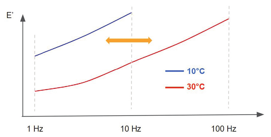
From a molecular point of view, polymer chains exhibit similar behavior when a deformation or a force is applied, the latter being both temperature- and frequency-dependent. As an example, for a polymer submitted to a constant load, E′ decreases over time because the polymer rearranges its chains in order to decrease the stresses applied. This explains why the modulus of elasticity is lower at low frequencies.
On the other hand, increasing the temperature (which corresponds to providing energy to the system) leads to an acceleration of chain motion in polymers and their rearrangement when submitted to a mechanical stimulus. From this, one understands that decreasing frequency leads to similar effects on the viscoelastic properties as increasing the temperature. Of course, the opposite is also true: increasing the frequency corresponds to decreasing the temperature.
In other words, increasing the frequency of mechanical solicitation on a specimen studied by DMA has the same effect on E’, E’’ and Tan δ as decreasing the temperature.
A DMA+ from Alpha Metravib is able to perform tests up to 1000 Hz, and the temperature range is between −150°C and 500°C. Based on these specifications, in order to study the viscoelastic properties of materials above 1000 Hz, it is necessary to perform frequency sweeps at different temperatures and use the frequency–temperature equivalence to simulate very high and very low frequencies.
Preliminary Tests
Before going further into parameter settings, there are two very important points (or rules, to some extent) to consider before building the master curve.
The first point is to remain within the linear domain of the material. As a reminder, the linear domain corresponds to a strain amplitude for which the viscoelastic properties remain constant with strain. In other words, the force applied during the test must be low enough to avoid inducing large molecular rearrangements in the polymer matrix.
Technically, in order to satisfy this first requirement, it is necessary to perform a strain sweep prior to building the master curve (an example is given in the Results section; see Figure 5) to define the linear domain.
The second point is to define the thermal profile of the viscoelastic properties. As stated previously, a master curve is built by combining frequency sweeps performed at different temperatures. If there is insufficient data, the master curve construction will be more difficult and most likely incomplete.
From the lowest to the highest temperature, it is therefore important to consider how much the viscoelastic properties change between each temperature step and to set the parameters accordingly. In particular, during the glass transition, E′, E’’ and Tan δ vary significantly, making it important to increase the number of frequency sweeps performed within this transition region.
For this reason, it is highly recommended to perform a temperature sweep before building the master curve, in order to define the temperature range of the glass transition. As for the first point described above, an example is provided in the Results section (see Figure 6).
The WLF law is applicable for reference temperatures above Tg: Tg < reference temperature < Tg + 100°C
FREE DOWNLOAD
Introduction to Dynamic Mechanical Analysis for Rubber Materials
Building Master Curves
Technically, the first step in building a master curve is to perform successive frequency sweep tests at different stabilized temperatures (details are given in the Methods section). The frequency sweeps are then horizontally shifted toward a reference temperature, usually corresponding to one of the frequency sweep curves performed.
Vertical shifting of the curves is also possible when building a master curve; however, this approach is not discussed in this article. Figure 3 illustrates the process used to construct a complete master curve.
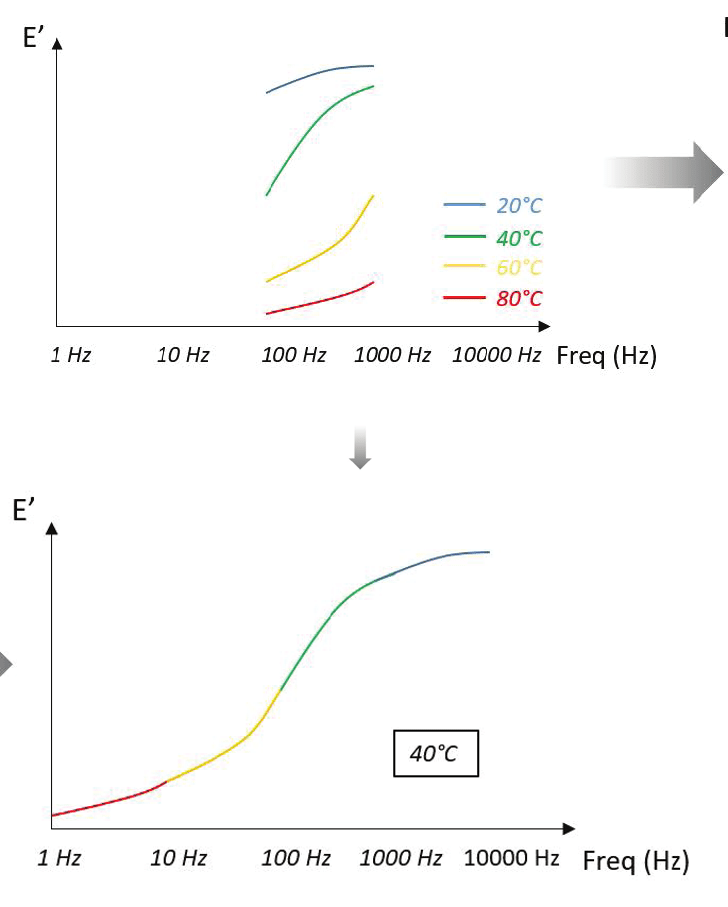
This process can be performed automatically using the Dyna+ software, or manually using a spreadsheet program.
WLF Model
The degree of horizontal shifting required to align the frequency sweeps with the reference curve can be determined as a function of temperature. Generally, two models are used to build the master curve.
The Williams–Landel–Ferry (WLF) relation, based on the principle of time–temperature superposition, is the most commonly used model. It is particularly well suited for temperatures close to the glass transition temperature and is favored for its flexibility. The WLF model describes the variation of the shift factor with temperature, as shown below.
WLF Model: log(aₜ) = − C₁(T − T₀) / [C₂ + (T − T₀)]
In this formulation, aₜ is the shift factor, T is the temperature, T₀ is the reference temperature, and C₁ and C₂ are two positive constants that depend on the material and the chosen reference temperature.
In other words, determining C₁ and C₂ allows the shift factor to be calculated (see Figure 8 in the Results section). Once the shift factor is known, any curve measured at temperature T can be shifted relative to the reference curve at T₀.
Arrhenius Model
The other model used to determine shift factors as a function of temperature is the Arrhenius model. The relationship between the shift factor and temperature can be described using the equation shown below.
Arrhenius Model: log(aₜ) = − (Eₐ / 2.303R) × (1/T − 1/T₀)
In this formulation, Eₐ is the activation energy, R is the universal gas constant (8.31 J·mol⁻¹·K⁻¹), T is the temperature, and T₀ is the reference temperature.
The Arrhenius law is well suited to describing polymer behavior below the glass transition temperature and applies effectively to secondary transitions. It is also useful for determining the activation energy associated with the glass transition.
FREE DOWNLOAD
Introduction to Dynamic Mechanical Analysis for Rubber Materials
Materials & Methods
Specimens
Rubber materials were studied using a DMA+1000 in film shear mode. A rubber film was prepared with the following dimensions:
- Length: 50 mm
- Width: 11.27 mm
- Thickness: 2 mm
Methods
A sinusoidal waveform is applied to the specimen at different frequencies (see Figure 4) and at different temperatures. To study the specimens, the shear film mode was used.
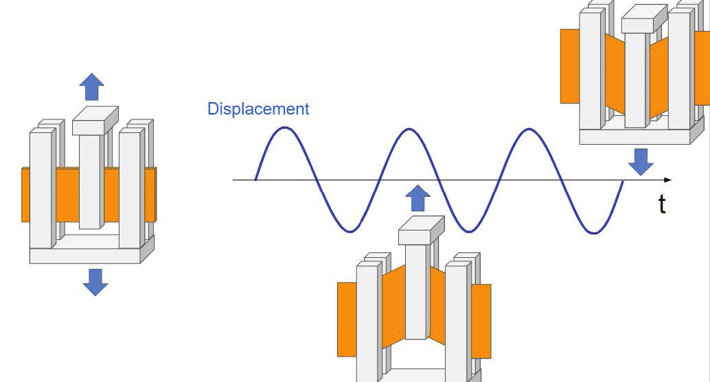
A dynamic displacement is applied to the specimen, and shear is applied to the two parts of the specimen between the specimen holder jaws. One of the advantages of this method is that no static load is necessary to maintain the specimen in the specimen holder.
The specimen must have a form factor that complies with the dimensioning rules for the excitation mode and must exhibit a stiffness variation range compatible with the instrument’s measurable stiffness range.
Moreover, it is important to use a homogeneous (no copolymers), isotropic, and amorphous specimen, and to ensure that no structural changes occur over the characterization temperature range (e.g., post-firing or decomposition).
The following tables show the different parameters used for the two preliminary tests and for the Master Curve itself.
Table 1. Strain Sweep Setting Parameters
| Dynamic | Force from 0.01 to 50 N |
|---|---|
| Frequency | 1 Hz |
| Static | — |
| Temperature | Room temperature |
Table 2. Temperature Sweep Setting Parameters
| Dynamic displacement | 5 µm |
|---|---|
| Frequency | 1 Hz |
| Static load | — |
| Temperature | From −100°C to 80°C, at 2°C/min |
Table 3. Frequency Sweep / Master Curve Setting Parameters
| Dynamic displacement | 5 µm |
|---|---|
| Frequency | From 1 Hz to 100 Hz |
| Static load | — |
| Temperature | 15 minutes stabilization at −75°C, followed by a frequency sweep. The process is repeated at −70°C, −65°C, −60°C, −55°C, −50°C, −45°C, −40°C, −35°C, −30°C, −25°C, −20°C, −15°C, −10°C, −5°C, 0°C, and 10°C. |
Results
Preliminary Strain Sweep Results
Figure 5 shows the modulus of elasticity G′ and Tan δ as a function of displacement at 1 Hz and room temperature. The graph clearly shows that the linearity domain is obtained for strain values below 0.05% (which corresponds to a 5 µm displacement). Above this range, the modulus decreases, and these changes are correlated with the nonlinear domain.
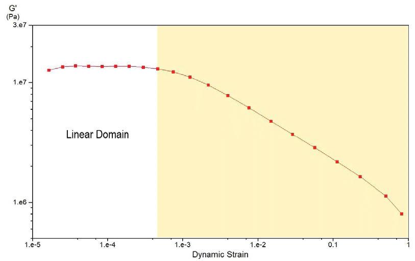
To build a proper master curve, the experiment must be performed within the linearity domain; otherwise, the curve superpositions are meaningless.
Preliminary Temperature Sweep Results
Figure 6 presents G’ and Tan δ as a function of temperature. The decrease in modulus with increasing temperature and the tan δ peak at −41.17°C are characteristic of a glass transition in the rubber.
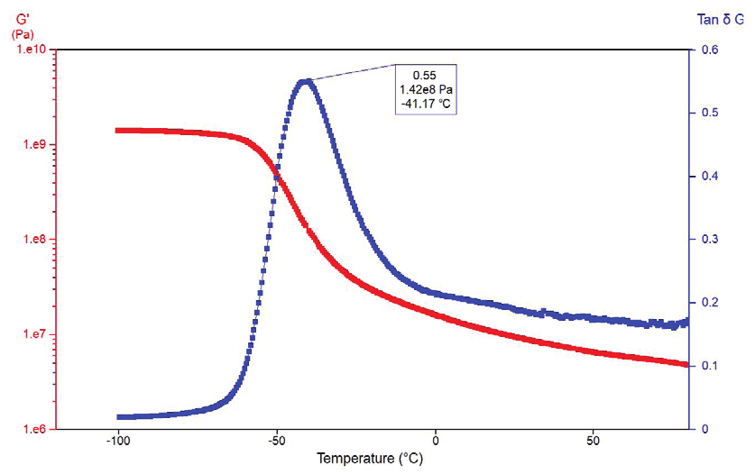
During this transition, a gradual and reversible change occurs in amorphous materials, from a hard and relatively brittle “glassy” state to a viscous or rubbery state as the temperature increases.
This information is important for setting up the master curve experiment, because more data are required around the glass transition temperature. In other words, additional frequency sweeps must be performed near the glass transition temperature in order to obtain sufficient data to construct the master curve.
Building the Master Curve
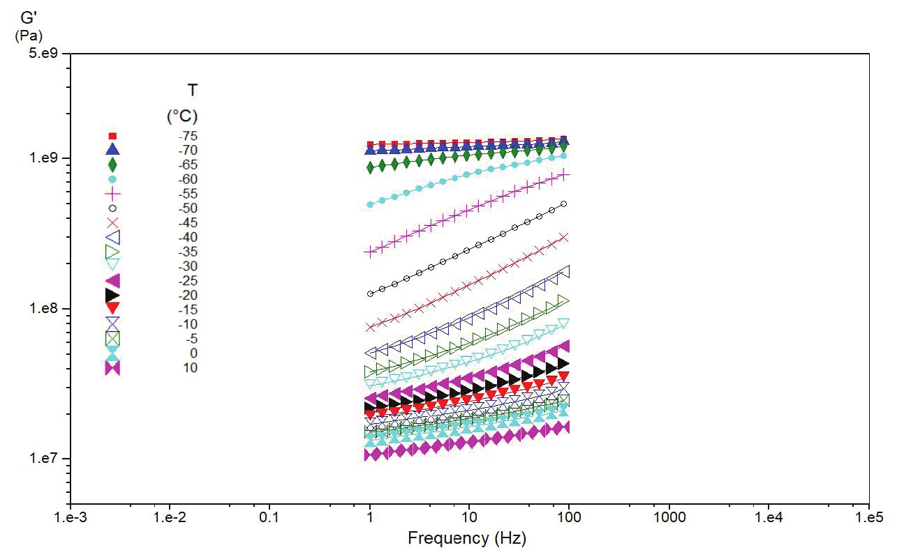
From the results obtained, frequency sweeps were performed between −75°C and 10°C, and from 1 Hz to 100 Hz at each temperature step. Figure 7 shows E′ as a function of frequency at different temperature steps; each curve can be shifted in order to build a master curve. As expected, the modulus increases slightly with frequency and decreases with temperature.
The computation performed by the DMA+ software allows the shift factor to be obtained as a function of temperature (Figure 8, with −30°C as the reference temperature). A shift factor of 1 means that there is no shift at this temperature, which is expected since −30°C is the reference.
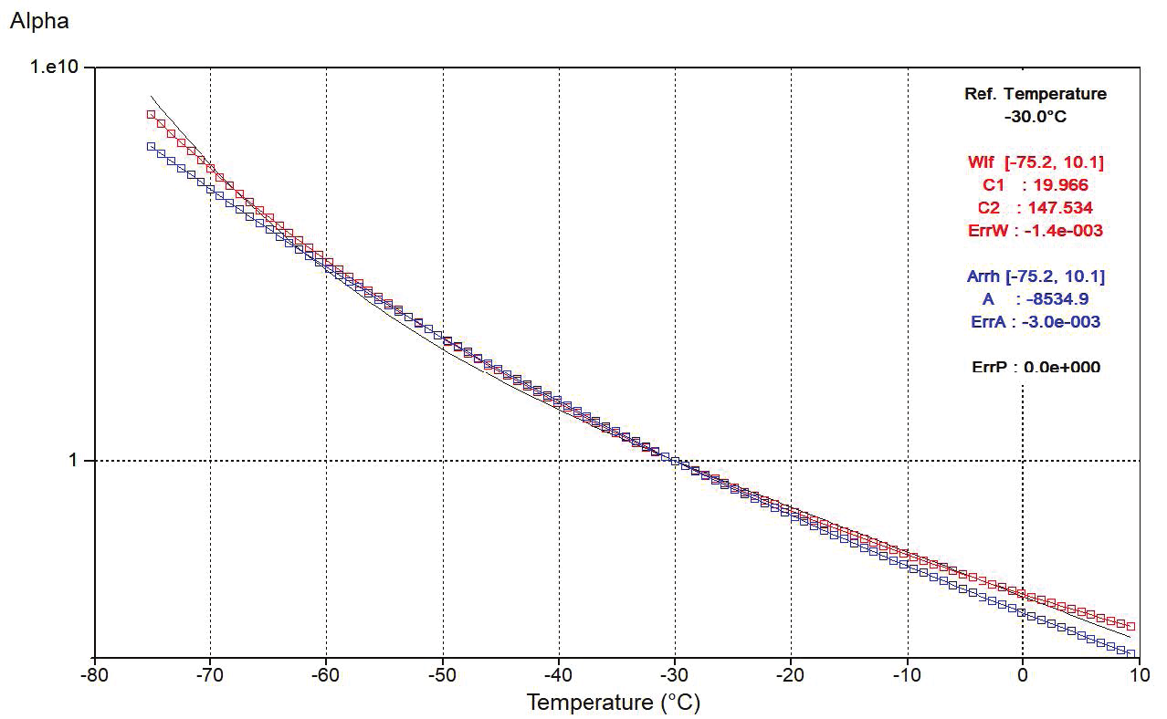
The further the shift factor deviates from 1, the more significant the shift. As shown in the graph, both the WLF and Arrhenius models are used to fit the results (see equations in the previous section). The values C₁ and C₂ for the WLF model and A for the Arrhenius model are not provided merely for information, but primarily to allow the user to reconstruct the master curve using a spreadsheet program.
Because the error between Arrhenius and the WLF model is in favor of the WLF model (see Figure 8), the fit is based on the empirical relationship of Williams-Landel-Ferry (WLF Model), with the following parameters obtained from the DMA+ software:
- C1 = 19.966
- C2 = 147.534
- Error = 2 × 10⁻³
Figure 9 shows the master curve built from the combination of all frequency sweeps (Figure 7), shifted using the aₜ values shown in Figure 8. Figure 9 presents the extrapolated viscoelastic properties G′ (red squares), G’’ (blue squares), and the polynomial fit (black line) as a function of frequency.
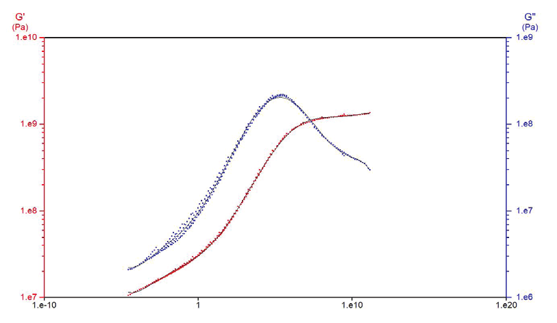
The variations in G′ and G’’ as a function of frequency are similar to those observed during a temperature sweep (see the Preliminary Tests section), and G’’ is correlated with relaxation times. Moreover, these results highlight the capability of the master curve to predict material properties over a wide frequency range (in this example, from 10⁻⁵ to 10¹⁰ Hz).
In Figure 9, all curve shifting was performed automatically using the Dyna+ software from Metravib Material Testing.
Conclusions
KEY TAKEAWAY
Frequency–temperature superposition enables prediction of viscoelastic behavior over frequency ranges beyond direct DMA measurement.
LEARN MORE ABOUT DMA
Introduction to Dynamic Mechanical Analysis for Rubber Materials
How rubber engineers evaluate real world material behavior
Inside the guide: guidance for improving analysis quality and useful direction for integrating DMA into research, development, and testing workflows.